Multiview Stereo Evaluation
The goal of this study is to provide high quality
datasets with which to benchmark and evaluate the performance of multiview
stereo algorithms. Each dataset is registered with a "ground-truth" 3D
model acquired via a laser scanning process, to be used as a baseline for
measuring accuracy and completeness (the ground truth is not distributed).
Data sets
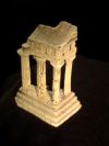 |
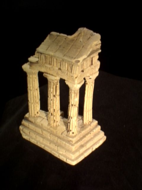
The object is a plaster reproduction of "Temple
of the Dioskouroi" in Agrigento, Sicily.
Click on thumbnail for a full-sized (640x480) image.
Resolution of ground truth model: 0.00025m (you may wish to
use this resolution
for your reconstruction as well) |
| "Temple"
data set (77 Mb): 317 views sampled on a hemisphere |
"TempleRing" data set (11 Mb): 47
views sampled on a ring around the object
(be sure not to use images or visual hull from the
"Temple" data set in any of your
computations
for "TempleRing" dataset) |
"TempleSparseRing"
data set (4 Mb): 16 views sampled on a ring around the object
(be sure not to use images or visual hull from the
other temple data sets in any of your
computations
for "TempleSparseRing" dataset) |
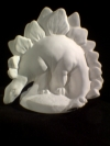 |
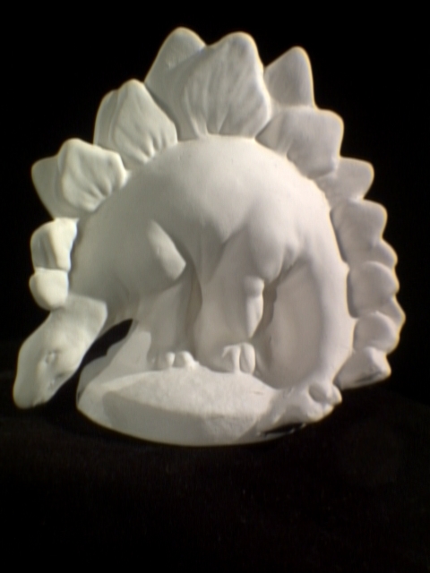
The object is a plaster dinosaur (stegosaurus).
Click on thumbnail for a full-sized (640x480) image.
Resolution of ground truth model: 0.00025m (you may wish to
use this resolution
for your reconstruction as well) |
| "Dino"
data set (83 Mb): 363 views sampled on a hemisphere |
"DinoRing" data set (11 Mb): 48
views sampled on a ring around the object
(be sure not to use images or visual hull from the
"Dino" data set in any of your
computations
for "DinoRing" dataset) |
"DinoSparseRing"
data set (4 Mb): 16 views sampled on a ring around the object
(be sure not to use images or visual hull from the
other dino data sets in any of your
computations
for "DinoSparseRing" dataset) |
Instructions on what to Submit:
(click here)
Calibration Accuracy
Calibration accuracy on these datasets appears to be on the order of a pixel
(a pixel spans about 1/4mm on the object). It is difficult to quantify the
calibration accuracy because we don't have point correspondences in all views.
However, when the images are reprojected onto the laser scanned mesh
reconstruction and averaged, 1-2 pixel wide features are clearly visible.
Some images and regions of the object are a bit out of focus, due in part to the
limited depth of field afforded by the imaging configuration. This is
probably a blessing in disguise, as it helps compensate for the lack of
sub-pixel registration. While there is certainly room for improvement, we
expect that this degree of accuracy will enable good results for most
algorithms.
Note that the images have been corrected to remove
radial distortion.
Data Acquisition
The images were captured using the
Stanford Spherical
Gantry which enables moving a camera on a sphere to specified
latitude/longitude angles. To calibrate the cameras, we took images of a
planar grid from 68 viewpoints and used a combination of
Jean-Yves
Bouguet's matlab toolbox and our own software to find grid points and
estimate camera intrinsics and extrinsics. From these parameters, we
computed the gantry radius and camera orientation, hence enabling us to map any
gantry position (specified as a latitude/longitude pair) to a complete set of
camera parameters. We then scanned the object from several orientations
using a Cyberware Model 15 laser scanner and merged the results using
vrip. The
cameras were aligned with the resulting mesh using software written by Daniel
Azuma and Daniel Wood plus some additional routines that we wrote. Whew!
We sampled up to 395 viewpoints on a full hemisphere. However, in
certain configurations, the gantry cast shadows on the object and these images
had to be manually removed. We found that 40% of the images contained
shadows. To limit the dropouts from shadows, we covered the hemisphere
twice, with two different arm configurations, for a total of 790 views.
Using this strategy, we were able to get non-shadowed images for a majority
of the hemisphere (e.g., 80% of the hemisphere for the "temple" data set).
File formats
Each dataset name contains the following:
| name*.png: |
images in
png format, a portable
lossless codec |
| name_par.txt: |
camera parameters. There is one line for each
image. The format for each line is:
"imgname.png k11 k12 k13 k21 k22 k23 k31 k32 k33 r11 r12 r13 r21 r22 r23
r31 r32 r33 t1 t2 t3"
The projection matrix for that image is K*[R t]
The image origin is top-left, with x increasing horizontally, y vertically |
| name_ang.txt: |
latitude, longitude angles for each image.
Not needed to compute scene->image mapping, but may be helpful for
visualization.
Note that (lat, lon) corresponds to the same image as (-lat, 180 + lon),
rotated 180 degrees in the image plane. The positive and negative
latitude images correspond to the two coverings of the hemisphere, as
described above, to avoid shadows. The -lat images appear
"upside-down" (in fact they're rotated 180 degrees). |
|
README.txt
|
information about the object, including
bounding box; in some cases, includes tips useful for computing visual
hull, if your algorithm needs it. |
Last Changed
October 23, 2005